|
|
|
Click on each of following figures to watch a larger view.
 Fig 1.
 Fig 2.
 Fig 3.
Fig. 1 Filling front positions and the Last Point to Fill (LPF) position
that does not coincide with the preset vent location without control
Fig. 2 Filling front positions and the LPF position that coincide
with the preset vent location with control
Fig. 3 The history of injection gate pressures achieving Fig. 2 under control
To top
Click on each of following figures to watch a larger view.
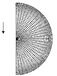 Fig 1.
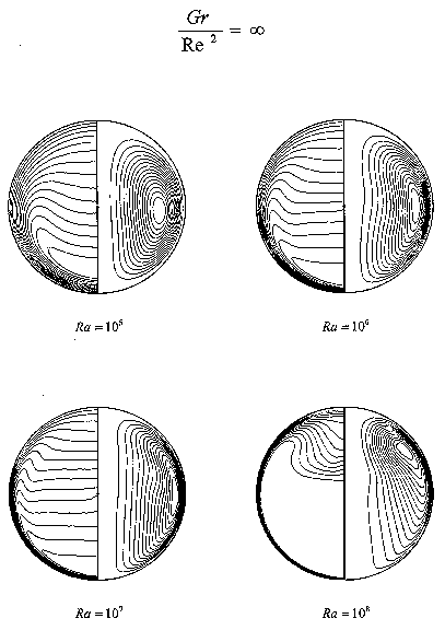 Fig 2.
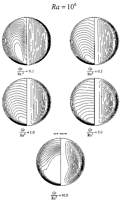 Fig 3.
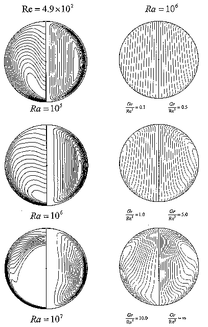 Fig 4.
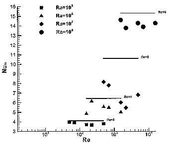 Fig 5.
Fig. 1 Schematic diagram of the computational grid system
Fig. 2 Pseudosteady-state streamline patterns and temperature field contours
corresponding to the Rayleigh number 105, 106,
107, and 108 within non-rotating spheres
Fig. 3 Pseudosteady-state streamline patterns and temperature field contours
corresponding to the Rayleigh number of 106 (Gr/Re2
=0.1, 0.5, 1, 5 and 10)
Fig. 4 Left coloum Pseudosteady-state streamline patterns and
temperature field contours corresponding to Re=4.9 × 10²
(Ra=105,106 and 107)
Right coloum Pseudosteady-state streamline patterns and
temperature field contours corresponding to Re=106
(Gr/Re2= 0.1, 0.5, 1, 5, 10 and ¥)
Fig. 5 Dependence of the mean Nusselt number on the Rayleigh and Reynolds numbers
To top
Click on each of following figures to watch a larger view.
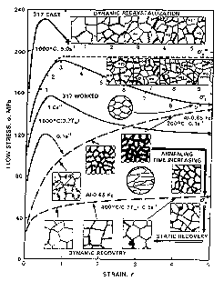 Fig 1.
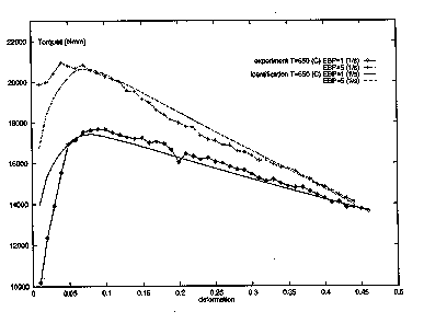 Fig 2.
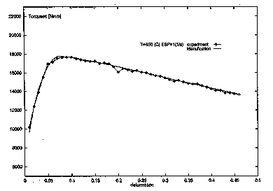 Fig 3.
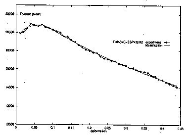 Fig 4.
 Fig 5.
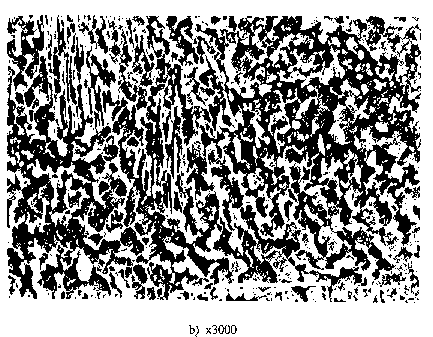 Fig 6.
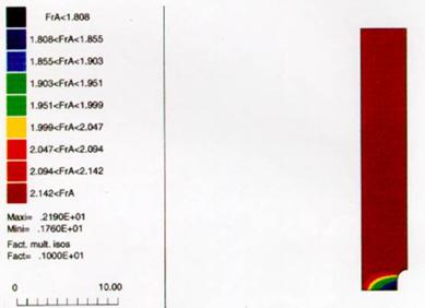 Fig 7.
Fig. 1 Flow curves corresponding to DRV (dash lines) and DRX (solid lines)
(Curtesy of J.J. Ionas et al, Treastise on Materials Science and Technology,
Vol. 6, Plastic Deformation of Materials, 394-490. Academic Press, New York, 1975)
Fig. 2 Torque versus deformation of experiment and calculation at 650°
C and nominal strain rates of 1 s-1 and 5 s-1
Fig. 3 Torque versus deformation of experiment and calculation at 650°
C and nominal strain rates of 1 s-1
Fig. 4 Torque versus deformation of experiment and calculation at 650°
C and nominal strain rates of 5 s-1 (Notice that when identification is performed
separately at strain rates of 1 s-1 (Fig. 3) and of 5 s-1 (Fig. 4),
the agreement is better than that obtained from identifying both simultanuously (Fig. 2))
Fig. 5 Simulation result of temperature distribution with constitutive equation proposed and parameters
identified at nominal strain rate of 5 s-1
Fig. 6 Microstructure of XC70 ([C]=0.65 - 0.73) after deformation at boundary area of the sample
Fig. 7 Size of substructure distribution simulated according to a formula proposed in the research
To top
Click on each of following figures to watch a larger view.
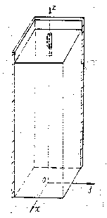 Fig 1.
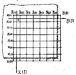 Fig 2.
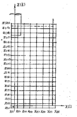 Fig 3.
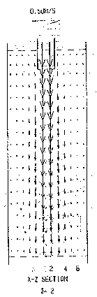 Fig 4.
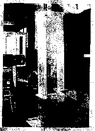 Fig 5.
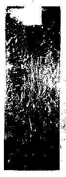 Fig 6.
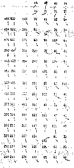 Fig 7.
Fig. 1 Computational domain (a quarter of the mold)
Fig. 2, 3 Computational grids
Fig. 4 One of the 2-D views of the folw fields from the simulations
Fig. 5 Experimental setup for the flow field measurement with LDA
Fig. 6 Snapshot of the flow field corresponding to Fig. 4
Fig. 7 The flow field from LDA corresponding to Fig. 4
Click on each of following figures to watch a larger view.
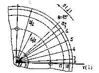 Fig 1.
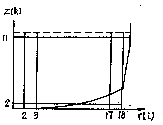 Fig 2.
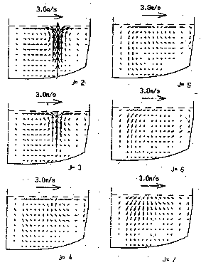 Fig 3.
Fig. 1, 2 Computaional grids
Fig. 3 Velocity field from the simulation
Click on each of following figures to watch a larger view.
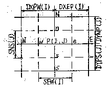 Fig 1.
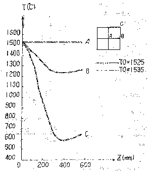 Fig 2.
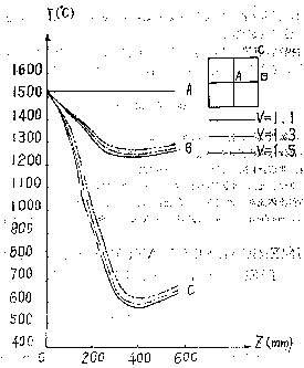 Fig 3.
Fig. 1 A control volume used in the calculation
Fig. 2 The effect from the temperature of the liquid metal in the tundish on the
temperature distribution inside the mold
Fig. 3 The effect of withdrawal rate on the temperature distribution inside the mold
Click on each of following figures to watch a larger view.
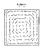 Fig 1.
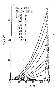 Fig 2.
 Fig 3.
Fig. 1 One of the simulated flow patterns under SEMS
Fig. 2 The effect of one operational factor from SEMS on the flow
Fig. 3 Relative change of flow energy versus the change of one operational factor
To top